Empirical Distribution Function and Quantiles
BIFIE.ecdf.RdComputes an empirical distribution function (and quantiles).
If only some quantiles should
be calculated, then an appropriate vector of breaks (which are quantiles)
must be specified.
Statistical inference is not conducted for this method.
Usage
BIFIE.ecdf( BIFIEobj, vars, breaks=NULL, quanttype=1, group=NULL, group_values=NULL )

# S3 method for class 'BIFIE.ecdf'
summary(object,digits=4,...)
Arguments
- BIFIEobj
Object of class
BIFIEdata- vars
Vector of variables for which statistics should be computed.
- breaks
Optional vector of breaks. Otherwise, it will be automatically defined.
- quanttype
Type of calculation for quantiles. In case of
quanttype=1, a linear interpolation is used (which istype='i/n'inHmisc::wtd.quantile), while forquanttype=2no interpolation is used.- group
Optional grouping variable
- group_values
Optional vector of grouping values. This can be omitted and grouping values will be determined automatically.
- object
Object of class
BIFIE.ecdf- digits
Number of digits for rounding output
- ...
Further arguments to be passed
Value
A list with following entries
- ecdf
Data frame with probabilities and the empirical distribution function (See Examples).
- stat
Data frame with empirical distribution function stacked with respect to variables, groups and group values
- output
More extensive output
- ...
More values
See also
Hmisc::wtd.ecdf,
Hmisc::wtd.quantile
Examples
#############################################################################
# EXAMPLE 1: Imputed TIMSS dataset
#############################################################################
data(data.timss1)
data(data.timssrep)
# create BIFIE.dat object
bifieobj <- BIFIEsurvey::BIFIE.data( data.list=data.timss1, wgt=data.timss1[[1]]$TOTWGT,
wgtrep=data.timssrep[, -1 ] )
#> +++ Generate BIFIE.data object
#> |*****|
#> |-----|
# ecdf
vars <- c( "ASMMAT", "books")
group <- "female" ; group_values <- 0:1
# quantile type 1
res1 <- BIFIEsurvey::BIFIE.ecdf( bifieobj, vars=vars, group=group )
#> |*****|
summary(res1)
#> ------------------------------------------------------------
#> BIFIEsurvey 3.8.0 ()
#>
#> Function 'BIFIE.ecdf'
#>
#> Call:
#> BIFIEsurvey::BIFIE.ecdf(BIFIEobj = bifieobj, vars = vars, group = group)
#>
#> Date of Analysis: 2026-01-11 08:35:25.359839
#> Time difference of 0.01169848 secs
#> Computation time: 0.01169848
#>
#> Multiply imputed dataset
#>
#> Number of persons = 4668
#> Number of imputed datasets = 5
#> Number of Jackknife zones per dataset = 0
#> Fay factor = 1
#>
#> Empirical Distribution Function
#> yval ASMMAT_female0 ASMMAT_female1 books_female0 books_female1
#> 1 0.00 289.4060 289.2616 1.0000 1.0000
#> 2 0.01 360.4102 350.5463 1.0000 1.0000
#> 3 0.02 378.2956 370.2925 1.0000 1.0000
#> 4 0.03 390.7284 382.2644 1.0000 1.0000
#> 5 0.04 398.2713 391.3413 1.0000 1.0000
#> 6 0.05 404.7193 399.0253 1.0000 1.0000
#> 7 0.06 410.9382 404.2058 1.0000 1.0000
#> 8 0.07 416.3854 409.1407 1.0000 2.0000
#> 9 0.08 420.9947 413.9343 1.0000 2.0000
#> 10 0.09 425.1791 418.1969 1.0000 2.0000
#> 11 0.10 429.8868 422.6586 1.0000 2.0000
#> 12 0.11 433.8429 425.8044 1.0000 2.0000
#> 13 0.12 437.6019 428.9276 1.0000 2.0000
#> 14 0.13 440.4902 432.0660 1.0855 2.0000
#> 15 0.14 443.2934 434.9671 2.0000 2.0000
#> 16 0.15 446.2611 437.8459 2.0000 2.0000
#> 17 0.16 449.0259 441.0204 2.0000 2.0000
#> 18 0.17 452.1626 443.5597 2.0000 2.0000
#> 19 0.18 454.5535 446.1485 2.0000 2.0000
#> 20 0.19 457.0869 448.4828 2.0000 2.0000
#> 21 0.20 458.9986 450.8571 2.0000 2.0000
#> 22 0.21 460.9323 453.0013 2.0000 2.0000
#> 23 0.22 462.7966 455.4279 2.0000 2.0000
#> 24 0.23 464.8803 458.1117 2.0000 2.0000
#> 25 0.24 466.9136 460.2872 2.0000 2.0000
#> 26 0.25 469.2726 462.6059 2.0000 2.0000
#> 27 0.26 471.2657 464.5962 2.0000 2.0000
#> 28 0.27 473.5467 466.6757 2.0000 2.0000
#> 29 0.28 475.4000 468.6851 2.0000 2.0000
#> 30 0.29 477.8102 470.4226 2.0000 2.0000
#> 31 0.30 480.0956 472.2576 2.0000 2.0000
#> 32 0.31 482.2891 474.2782 2.0000 2.0000
#> 33 0.32 484.0860 475.9431 2.0000 2.0000
#> 34 0.33 485.9087 477.6245 2.0000 2.4447
#> 35 0.34 487.6431 479.6084 2.0000 3.0000
#> 36 0.35 489.5604 481.2538 2.0000 3.0000
#> 37 0.36 491.2799 483.2301 2.0000 3.0000
#> 38 0.37 493.2986 484.8385 2.0000 3.0000
#> 39 0.38 495.0179 486.7814 2.0000 3.0000
#> 40 0.39 496.6917 488.4322 2.0000 3.0000
#> 41 0.40 498.2431 490.2857 3.0000 3.0000
#> 42 0.41 500.2859 492.0067 3.0000 3.0000
#> 43 0.42 501.9409 493.5864 3.0000 3.0000
#> 44 0.43 503.5877 495.2050 3.0000 3.0000
#> 45 0.44 505.3102 497.0009 3.0000 3.0000
#> 46 0.45 507.0328 498.5194 3.0000 3.0000
#> 47 0.46 508.6513 499.8466 3.0000 3.0000
#> 48 0.47 510.1753 501.5958 3.0000 3.0000
#> 49 0.48 511.8156 503.2402 3.0000 3.0000
#> 50 0.49 513.4574 504.9194 3.0000 3.0000
#> 51 0.50 514.8680 506.4329 3.0000 3.0000
#> 52 0.51 516.4589 507.9330 3.0000 3.0000
#> 53 0.52 518.0709 509.7049 3.0000 3.0000
#> 54 0.53 519.4852 511.5210 3.0000 3.0000
#> 55 0.54 520.8204 512.9131 3.0000 3.0000
#> 56 0.55 522.5602 514.5176 3.0000 3.0000
#> 57 0.56 524.3329 516.1179 3.0000 3.0000
#> 58 0.57 525.9907 517.9863 3.0000 3.0000
#> 59 0.58 527.8937 519.5515 3.0000 3.0000
#> 60 0.59 529.2754 521.1383 3.0000 3.0000
#> 61 0.60 530.7957 522.9874 3.0000 3.0000
#> 62 0.61 532.3495 524.4240 3.0000 3.0000
#> 63 0.62 534.0085 526.0524 3.0000 3.0000
#> 64 0.63 535.8988 527.7227 3.0000 3.0000
#> 65 0.64 537.9137 529.3551 3.0000 3.0000
#> 66 0.65 539.5138 531.0225 3.0000 3.0000
#> 67 0.66 541.2964 532.4859 3.0000 3.0000
#> 68 0.67 542.9439 534.1731 3.0000 3.0000
#> 69 0.68 544.7335 535.5444 3.0000 3.0000
#> 70 0.69 546.2788 537.1540 3.0000 3.0000
#> 71 0.70 548.0536 538.7727 3.0000 3.0000
#> 72 0.71 549.7821 540.3485 3.0000 3.0000
#> 73 0.72 551.8408 541.8885 3.0000 4.0000
#> 74 0.73 553.7181 543.8178 3.0000 4.0000
#> 75 0.74 555.4481 545.5449 4.0000 4.0000
#> 76 0.75 557.4563 547.2582 4.0000 4.0000
#> 77 0.76 559.2689 549.2598 4.0000 4.0000
#> 78 0.77 561.3302 550.8590 4.0000 4.0000
#> 79 0.78 563.8103 552.8609 4.0000 4.0000
#> 80 0.79 566.0606 554.5632 4.0000 4.0000
#> 81 0.80 567.8897 556.6981 4.0000 4.0000
#> 82 0.81 569.7978 559.0376 4.0000 4.0000
#> 83 0.82 571.6767 560.6622 4.0000 4.0000
#> 84 0.83 574.1766 562.9315 4.0000 4.0000
#> 85 0.84 576.3203 565.0438 4.0000 4.0000
#> 86 0.85 578.6383 567.4220 4.0000 4.0000
#> 87 0.86 580.9051 569.8376 4.0000 4.0000
#> 88 0.87 583.1823 572.2332 5.0000 4.0000
#> 89 0.88 585.9448 574.8882 5.0000 4.0000
#> 90 0.89 589.1086 578.0211 5.0000 5.0000
#> 91 0.90 591.7039 580.5636 5.0000 5.0000
#> 92 0.91 595.0740 583.8702 5.0000 5.0000
#> 93 0.92 598.3910 586.9706 5.0000 5.0000
#> 94 0.93 602.9135 589.8593 5.0000 5.0000
#> 95 0.94 607.5578 593.8227 5.0000 5.0000
#> 96 0.95 613.1091 597.9249 5.0000 5.0000
#> 97 0.96 618.9041 603.1582 5.0000 5.0000
#> 98 0.97 627.0231 609.0026 5.0000 5.0000
#> 99 0.98 637.2005 619.0757 5.0000 5.0000
#> 100 0.99 651.9489 629.8061 5.0000 5.0000
#> 101 1.00 720.2110 739.7378 5.0000 5.0000
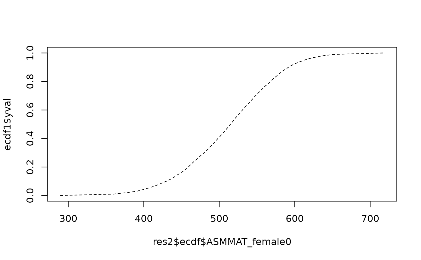
res2 <- BIFIEsurvey::BIFIE.ecdf( bifieobj, vars=vars, group=group, quanttype=2)
#> |*****|
# plot distribution function
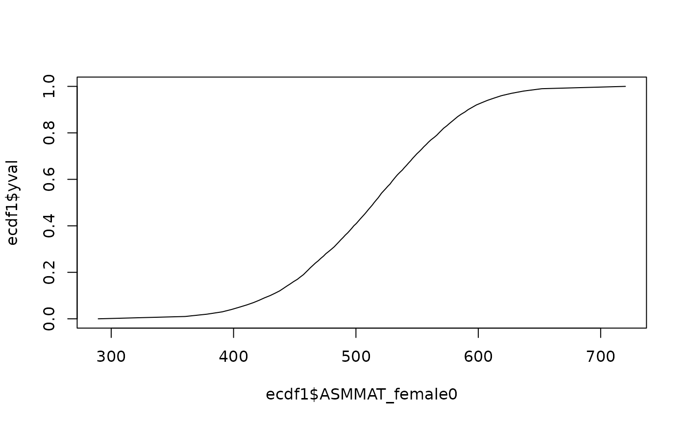
ecdf1 <- res1$ecdf
plot( ecdf1$ASMMAT_female0, ecdf1$yval, type="l")
 plot( res2$ecdf$ASMMAT_female0, ecdf1$yval, type="l", lty=2)
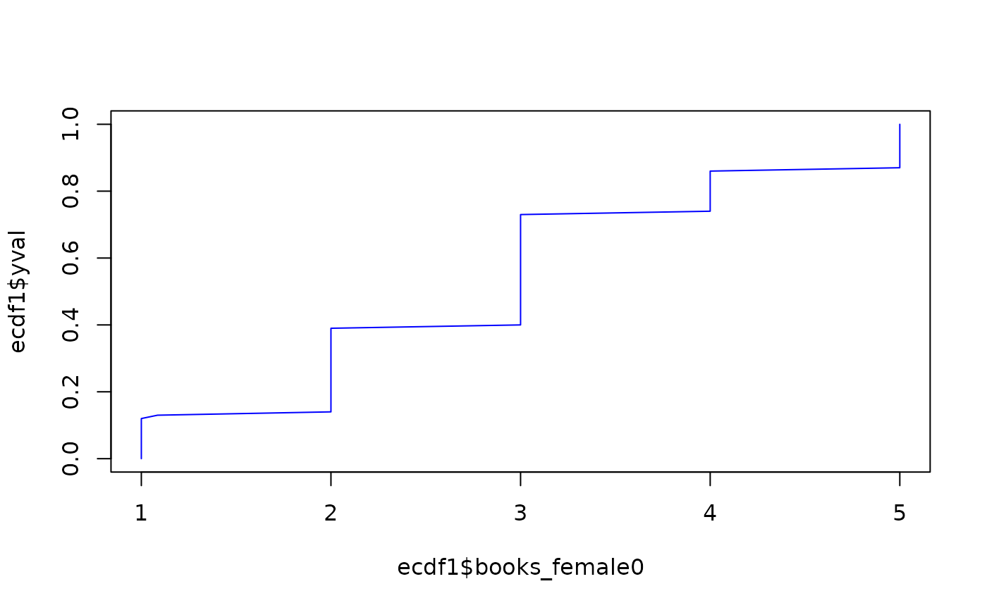
 plot( ecdf1$books_female0, ecdf1$yval, type="l", col="blue")